BAX visualizer

Overview

The BAX visualizer extension allows for an interactive graphical interpretation of the virtual measurement generated during a Bayesian Algorithm Execution (BAX) optimization run. Rather than modeling an explicit objective function, BAX builds a surrogate model from observations and executes a virtual algorithm on that model to decide where to sample next. The visualizer displays this virtual objective, its underlying samples, and how the algorithm converges over the course of the run.

Usage

The extension can be used both statically and dynamically during or after a Badger optimization run. When used during a Badger optimization, the plots will update at a set interval in real time according to the variables and plot options set. Any plot options, reference points, and variables are saved throughout the use of that instance of the BAX visualizer extension and are lost when the window is closed.

Constraints

The BAX visualizer extension is only available when conducting a Badger optimization that satisfies all of the following conditions:

• The optimization uses a BAX Generator.

• The routine has no objectives defined. BAX uses observations to visualize the optimization process, so it cannot be used with routines that have objectives defined. If objectives are present, remove them from the routine and try again.

• A routine is currently running or selected in the main Badger interface. If no routine is active, the extension will prompt you to start a routine first.

The controls shown within the extension additionally depend on which BAX algorithm the generator is configured to use. The supported algorithms are grid_optimize, pathwise_minimize_emittance, and pathwise_solenoid_alignment.

Tutorial

Step 1: Start Badger optimization

First step to use the BAX visualizer is to use the Badger UI to run through an optimization using a compatible BAX algorithm.

Once you have converged on a solution or have stopped the optimization after a certain number of iterations, you can visualize the virtual measurement and its convergence by opening the BAX visualizer extension.

Step 2: How to access the extension

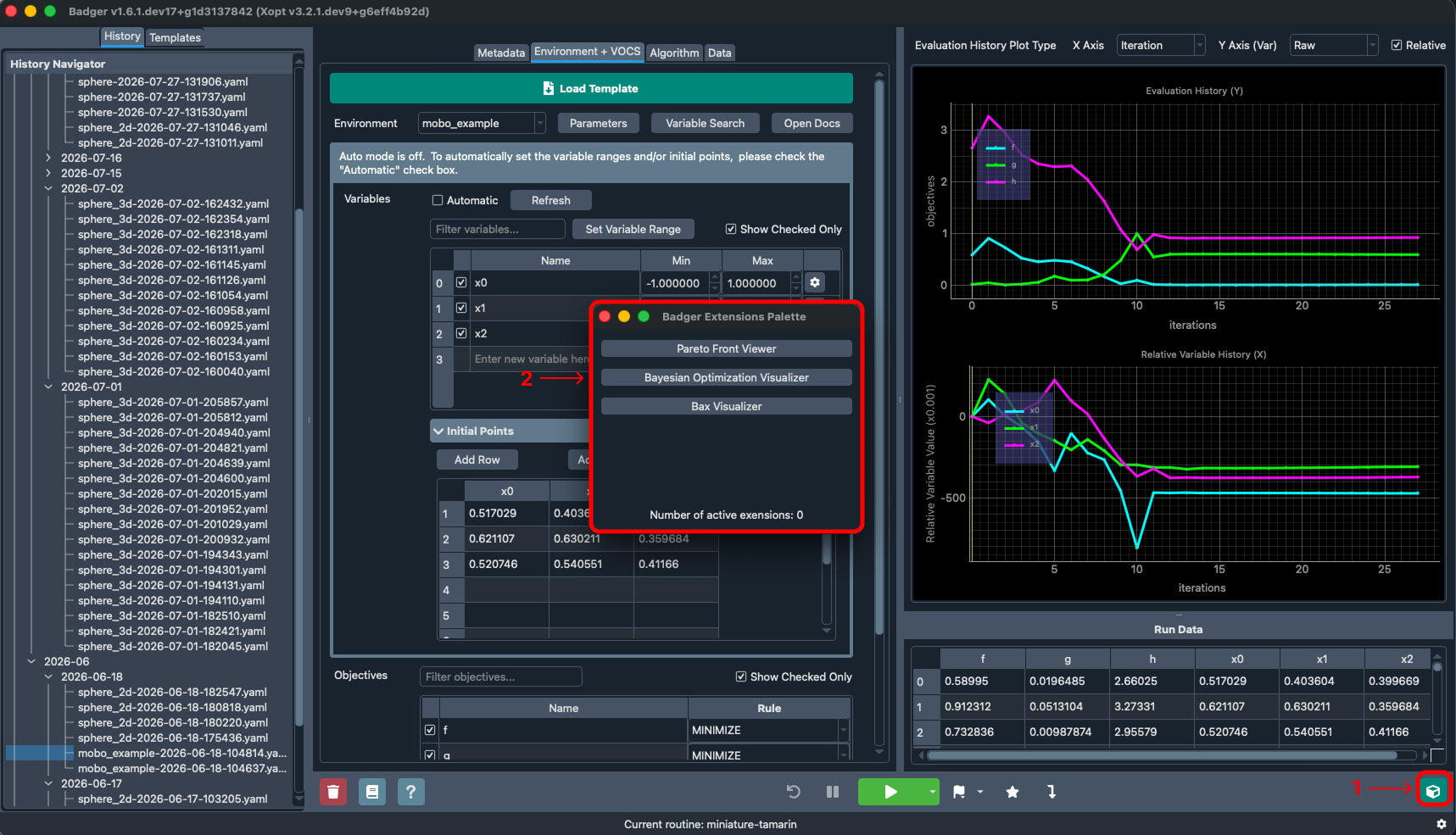
Description:

1 - Access the Badger extensions palette by clicking the icon in the bottom right

2 - The Badger extensions palette contains all extensions included by default with Badger Note: not all extensions are applicable to every optimization configuration

3 - Access the BAX visualizer extension by clicking the corresponding option within the Badger extensions palette

Step 3: BAX visualizer controls

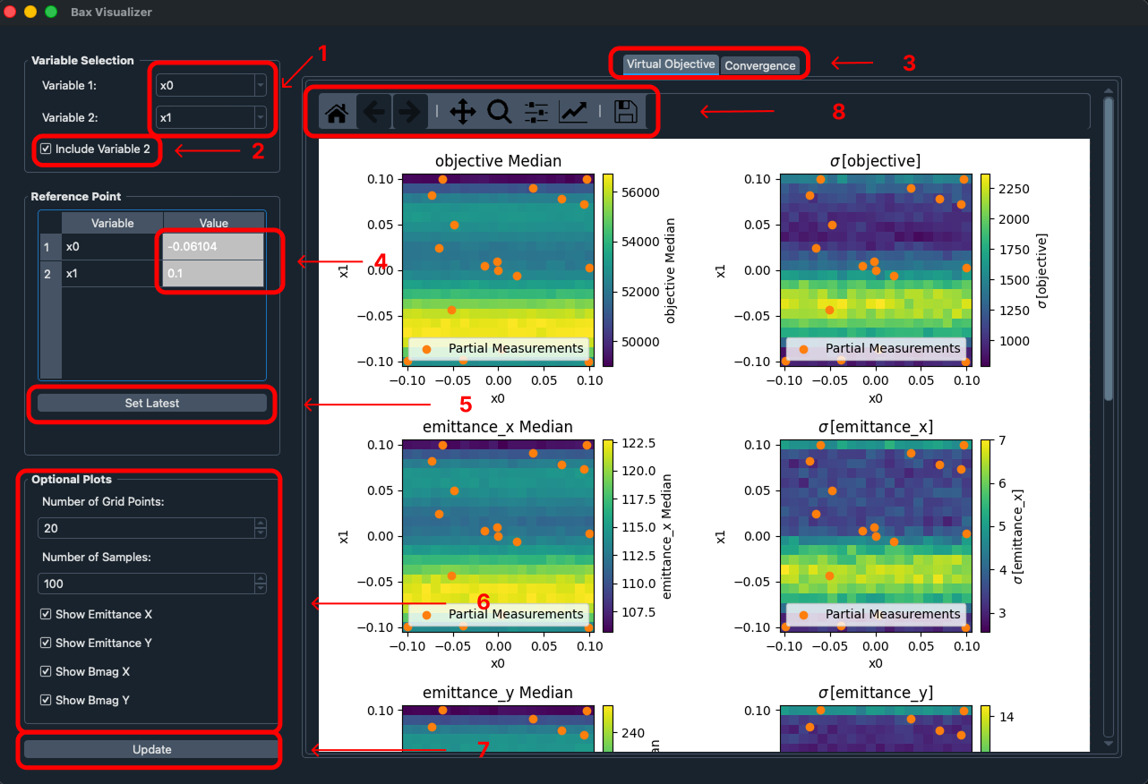
Description:

1 - Change the variables that are being plotted by the X and Y axes within the extension using the "Variable 1" and "Variable 2" selectors.

2 - By default the extension will plot two variables at a time. If you wish to only plot a single variable, you can uncheck the "Include Variable 2" option and the "Variable 2" selector will be disabled.

3 - At the top of the window you can toggle between the two different plot views: Virtual Objective and Convergence (see explanation below)

4 - The reference point table lists every variable in the routine alongside an editable reference value. This value is used to fix the input space for any axes that are not currently being visualized. The variables selected for the X and Y axes are grayed out and cannot be edited.

• Note: In >2D spaces the reference point determines the slice of the input space that is displayed for the axes that are not plotted.

5 - The "Set Latest" button will populate the reference point table with the most recently measured values from the optimization run, and the plots will update accordingly. The latest reference points are also shown in text below the button.

6 - You can control the resolution and sampling of the virtual measurement with the following options:

• Number of Grid Points - the number of mesh points used to visualize the surrogate model value. A higher number of points produces a higher resolution visualization, but at the cost of increased computation time (range: 10-100).

• Number of Samples - the number of virtual measurement samples drawn from the model at each grid point. A higher number of samples produces a smoother estimate at the cost of increased computation time (range: 10-1000).

Depending on the BAX algorithm in use, additional plot options let you toggle which results are displayed. These options appear only when applicable to the current algorithm:

• Show Objective - toggles the visualization of the virtual objective function (grid_optimize algorithm).

• Show Emittance X / Show Emittance Y - toggle the X and Y beam emittance metrics (pathwise_minimize_emittance algorithm).

• Show Bmag X / Show Bmag Y - toggle the X and Y beam mismatch (Bmag) components (pathwise_minimize_emittance algorithm).

• Show Alignment X / Show Alignment Y - toggle the X and Y solenoid misalignment metrics (pathwise_solenoid_alignment algorithm).

7 - The BAX visualizer extension will automatically update the charts reactively upon any changes to the controls above. If at any point you believe the plots are out of sync, you can forcefully rebuild them using the update button.

8 - The charts within the extension are interactive. Each plot includes the Matplotlib navigation toolbar, which allows you to pan, zoom, step back and forward through view states, reset to the home view, adjust the plot layout, and export the current plot as an image. When a chart is larger than the viewport it can be scrolled vertically.

Charts explanation

The BAX visualizer organizes its charts into two tabs.

Virtual objective

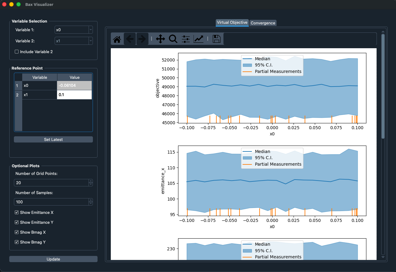
The "Virtual Objective" tab displays the surrogate model and the virtual measurement produced by the BAX algorithm.

• When plotting two variables, the chart shows the model predictions as contours across the selected X and Y axes, overlaid with the virtual measurement samples drawn from the model. The real observations used to train the model are shown as markers, and the current reference point is indicated on the plot.

• When only a single variable is selected (with "Include Variable 2" unchecked), the same information is displayed as a one dimensional plot of the surrogate value against the selected variable.

The display of results within this tab is controlled by the algorithm-specific plot options described in Step 3 (for example, the objective, emittance, Bmag, or alignment metrics).

Convergence

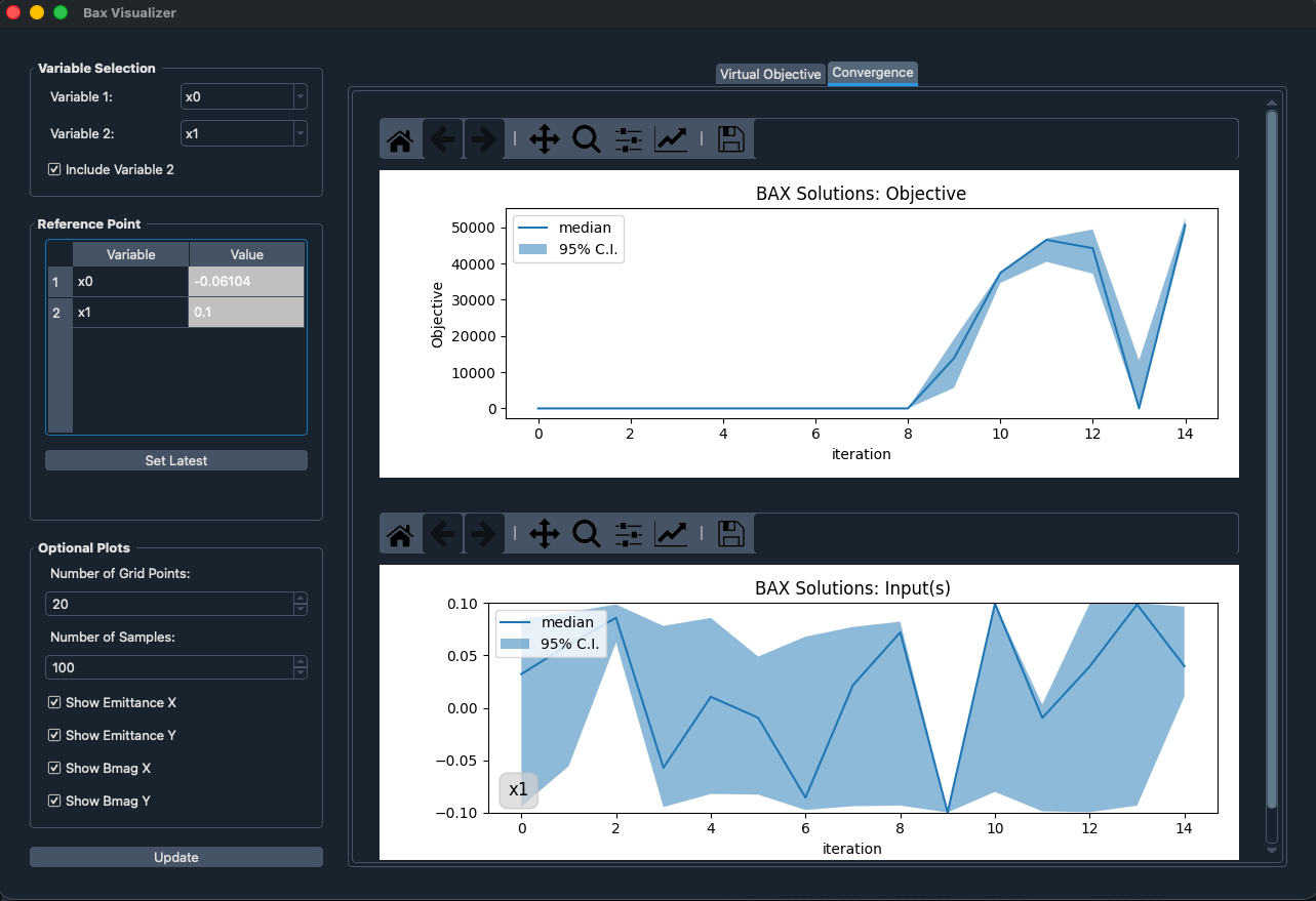
The "Convergence" tab contains two stacked plots that show how the BAX algorithm progresses across iterations of the optimization run.

• The objective convergence plot shows how the inferred objective value evolves as the optimization progresses.

• The input convergence plot shows how the recommended input values evolve as the optimization progresses.