GUI Usage
Once you launch Badger in GUI mode, you'll have various Badger features to explore. You can search through this page to get to the guide on any specify GUI feature, or if you believe a guide is missing for the topic you are interested in, please consider raising an issue here or shooting us an email, many thanks :)
GUI Layout
The Badger GUI is an interface made for optimizing accelerator performance. Behind the scenes, Badger uses Xopt, a python package designed to support a wide variety of control system optimization problems and algorithms. There are four important sections to defining an optimization problem using the Badger GUI: Environment, VOCS, Algorithm, and Metadata. The Badger GUI organizes these into three tabs, with Environment + VOCS being combined into a single main tab.
Environment + VOCS
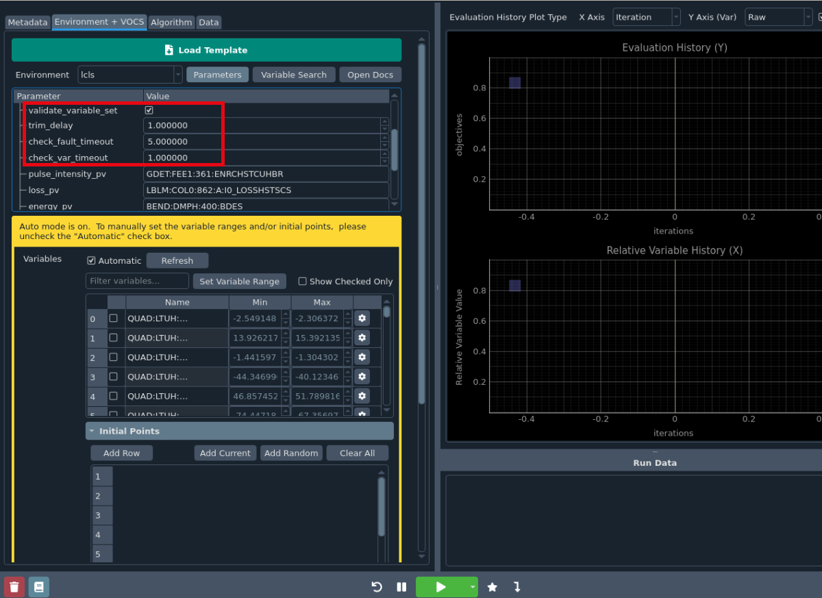
The Environment defines available variables and observables for a specific machine or control system. At SLAC, possible environments include LCLS, FACET, and LCLS_II. Each environment contains information about the variables available within that system, such as their bounds, along with operational parameters for data collection such as number of points, trim delay, fault timeout, and other information related to the interaction between the optimizer and the physical or simulated environment.
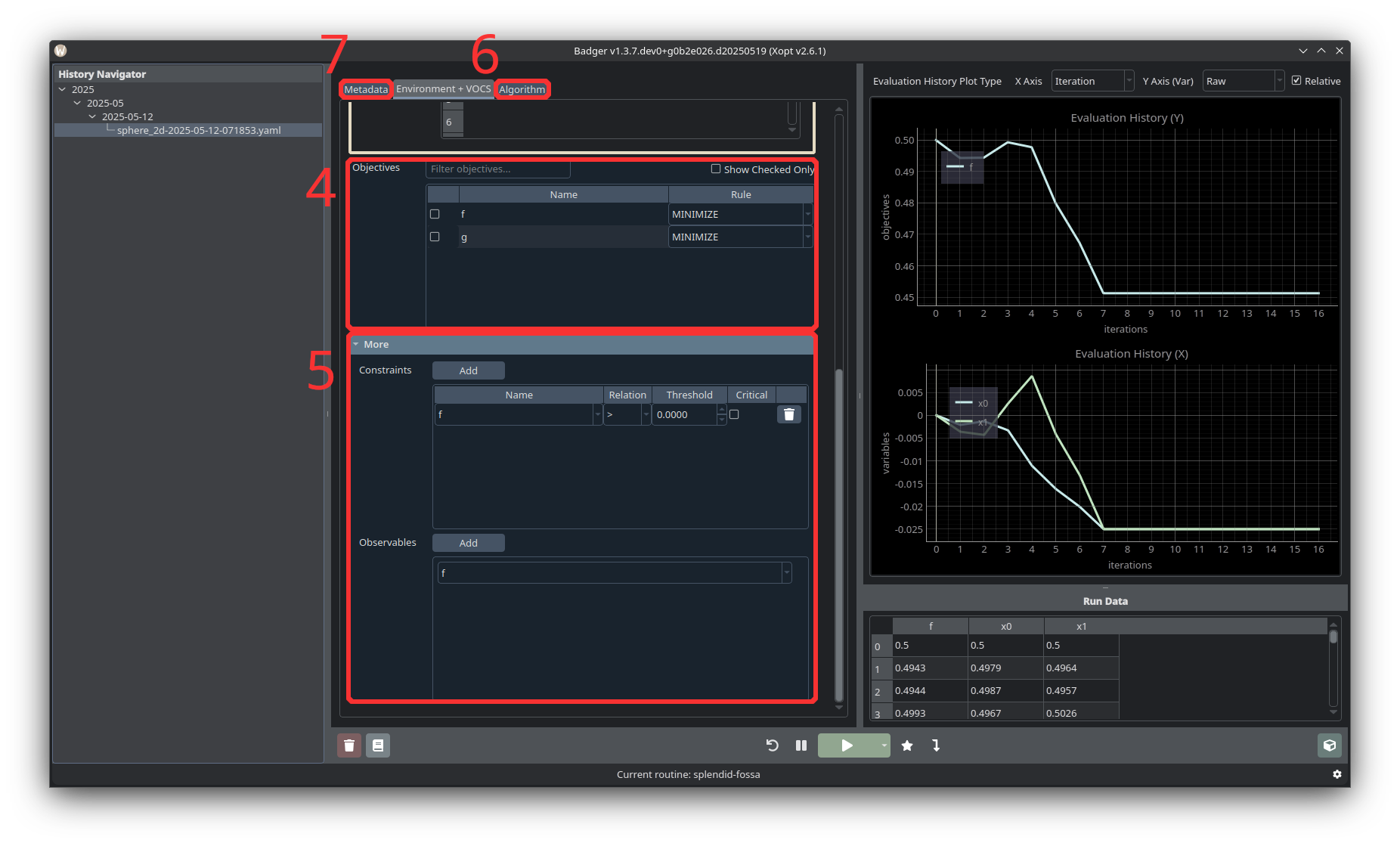
Within an environment, an optimization problem can be defined by selecting which variables to adjust, objectives to optimize, and any constraints to follow. VOCS represents the subset of variables, objectives, and constraints to be optimized within the environment. You can also add observables within the VOCS section, which the GUI will monitor and display but won’t otherwise interact with. The “Constraints” and “Observables” sections are optional for defining an optimization and are collapsed by default. They can be accessed by clicking on More at the bottom of the Environment + VOCS tab.
Loading a Template
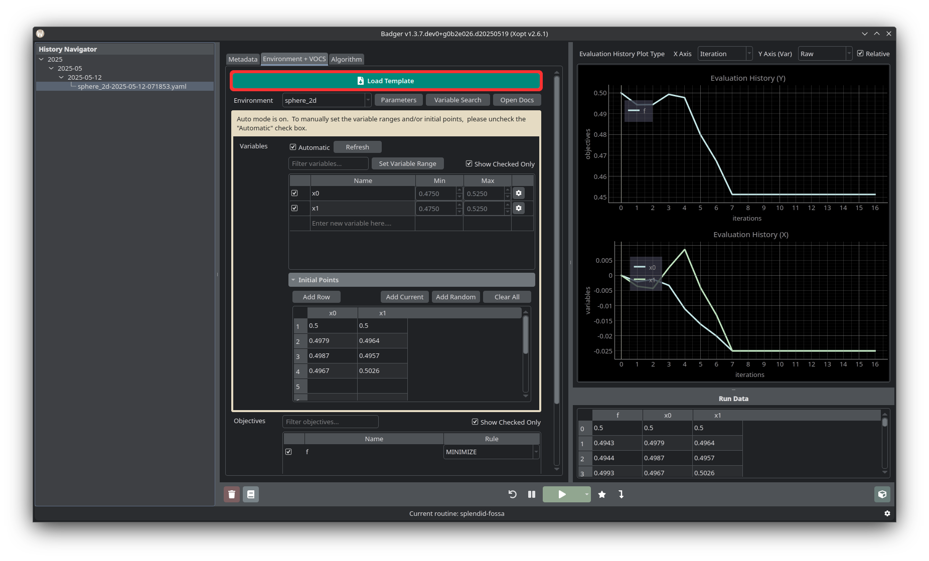
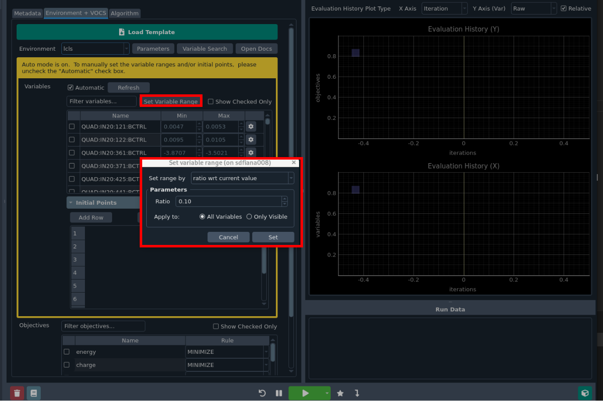
If there is already a template for the optimization you’d like to run, click the Load Template button at the upper left of the Environment + VOCS tab, and select the appropriate template. Make sure to check the environment parameters, variables and variable ranges, objectives, constraints/observables, and selected algorithm before running the optimization. See the templates page for more information about templates.
Run Buttons
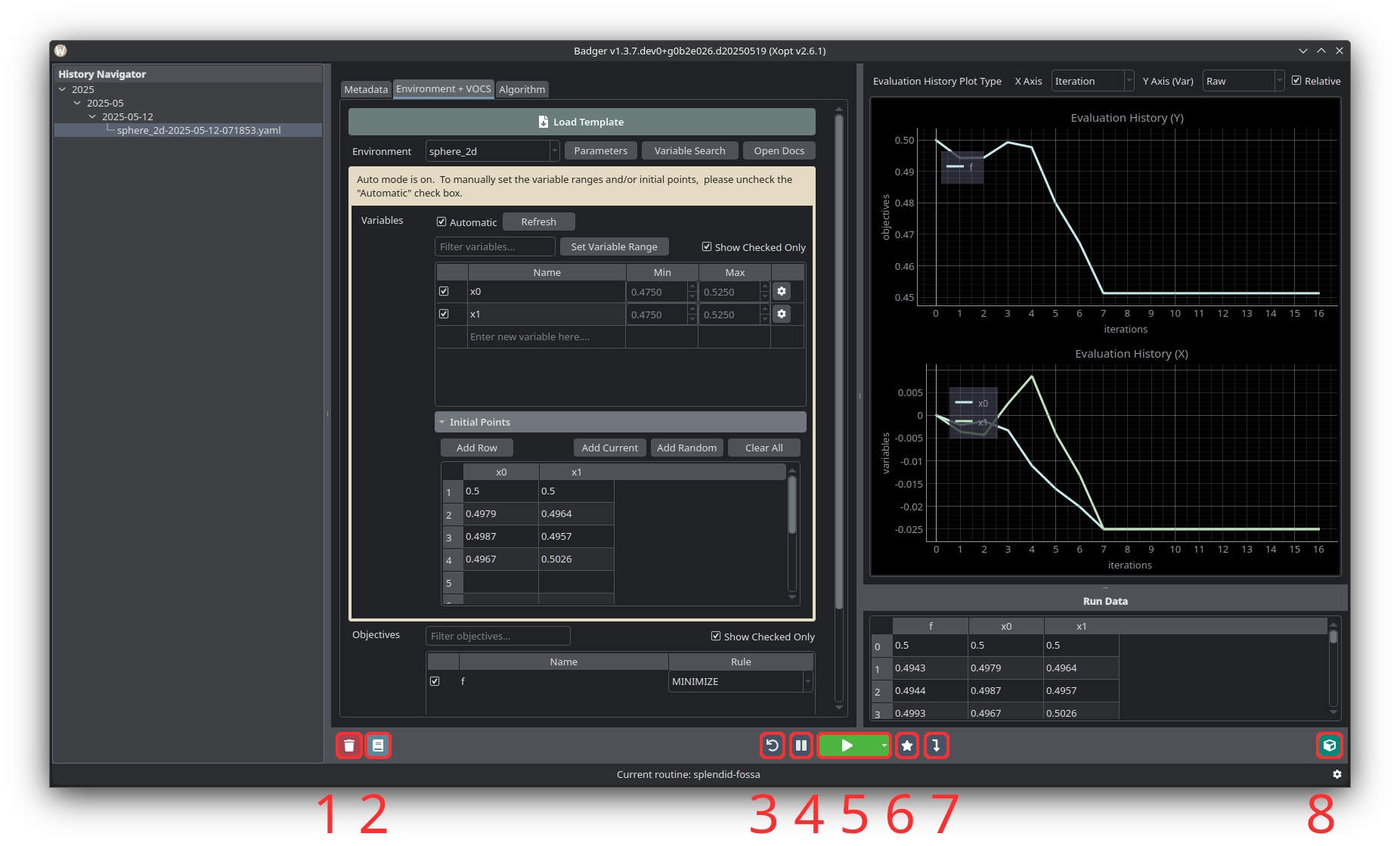
- Deletes the stored run data from the History Navigator and on disk.
- Save the current run's log to the configured logbook directory.
- Resets all variables to their values at the beginning of the run.
- Pause or resume the active run.
- Start or end a run.
- Jump to the optimal combination of variable values in the Plot Area.
- Set devices to the selected values.
- Open extension windows such as BOVisualizer and ParetoFrontViewer.
Plot Area and Run Data
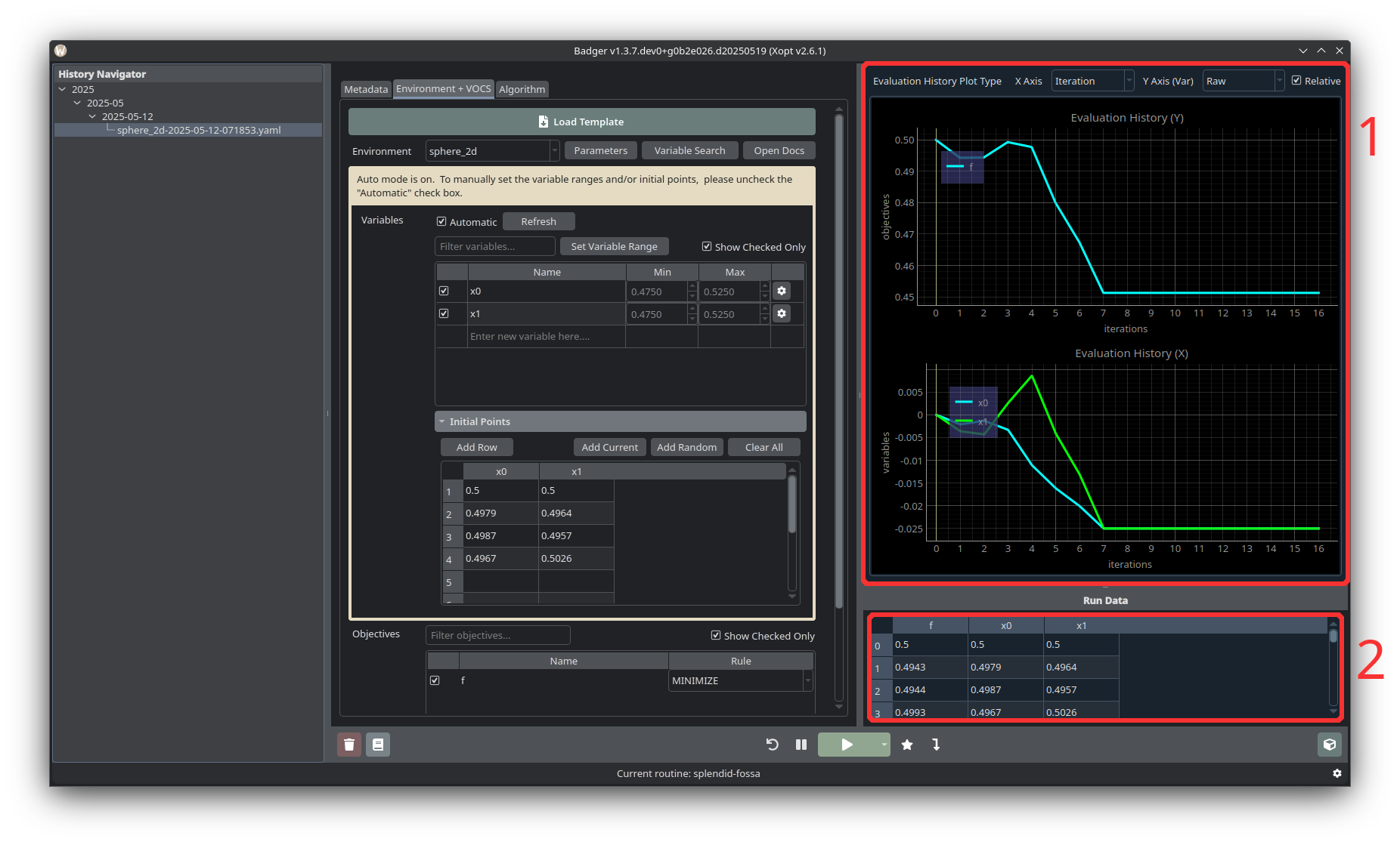
- Plot Area is where run data is visualized as a line graph.
- Run Data holds the raw data points which are fed into the plot.
History Navigator
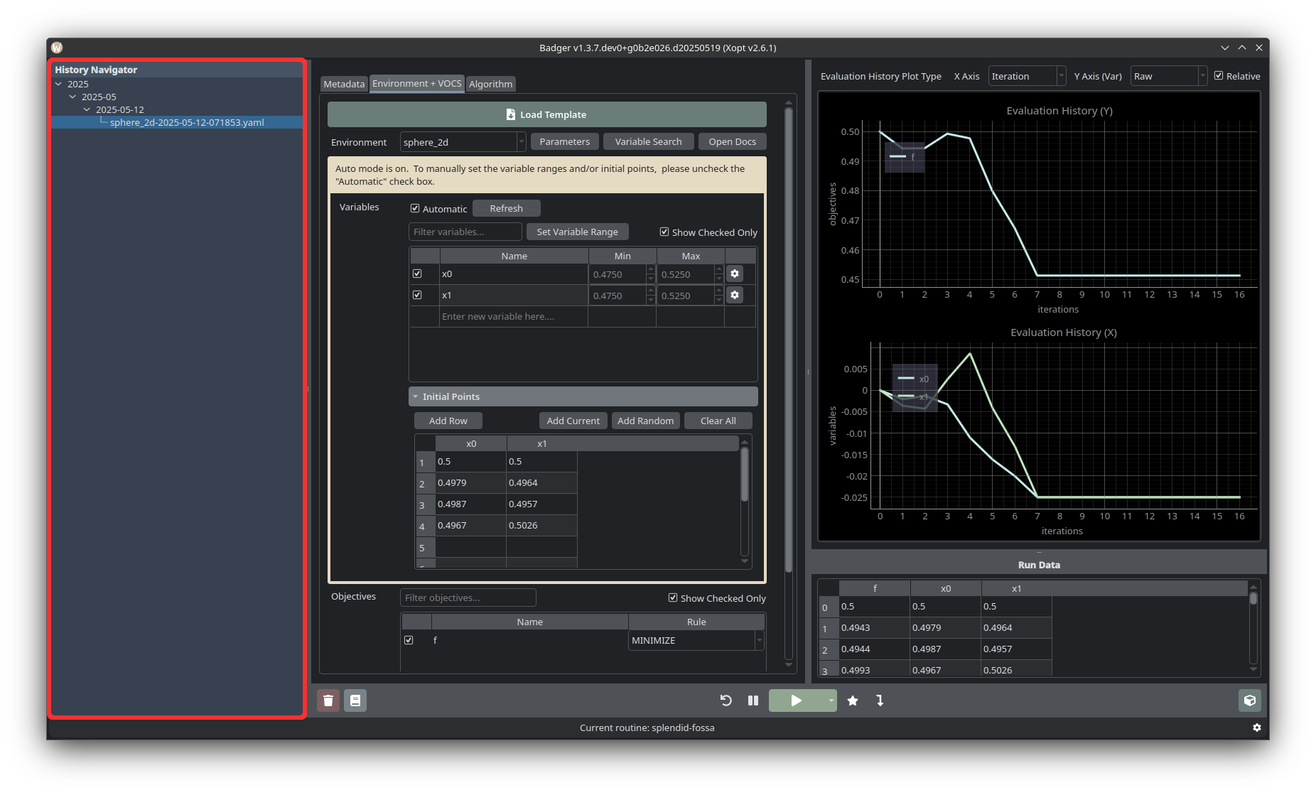
The History Navigator holds past runs, whose output can be loaded again with a single click on a given yaml file entry. Past runs are hierarchically organized by year, year and month, and year, month, and day, just like how they are organized in the Badger archive directory.
Algorithm
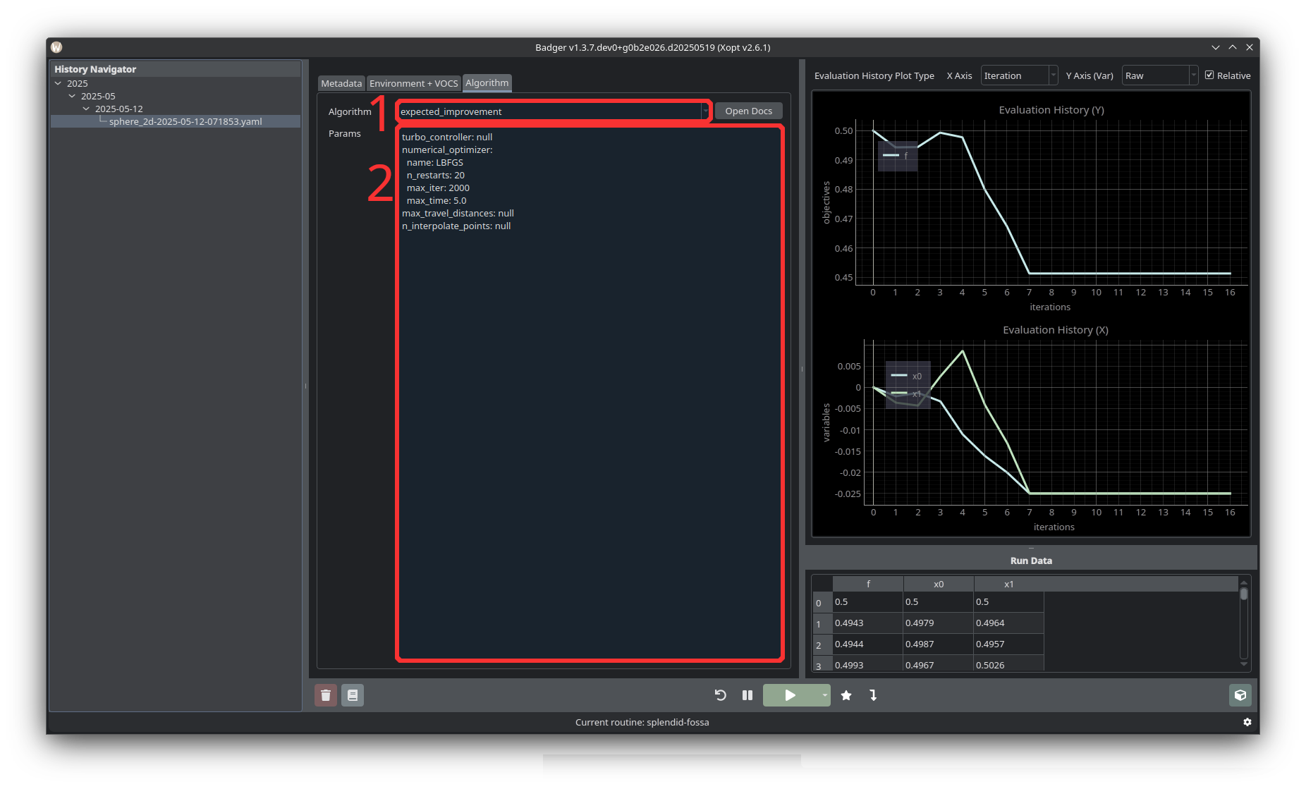
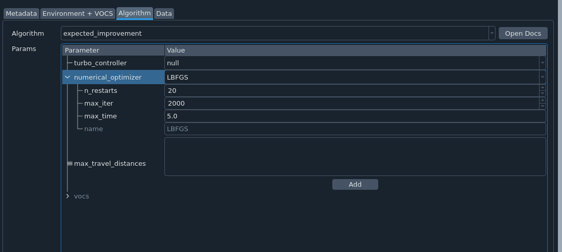
The Algorithm section lets you select an algorithm to use for optimization (1), as well as set the parameters of the selected algorithm (2). See “Overview of Different Optimization Algorithms” for a more detailed overview of different options. Common algorithms used at SLAC are expected improvement and nelder-mead.
Metadata
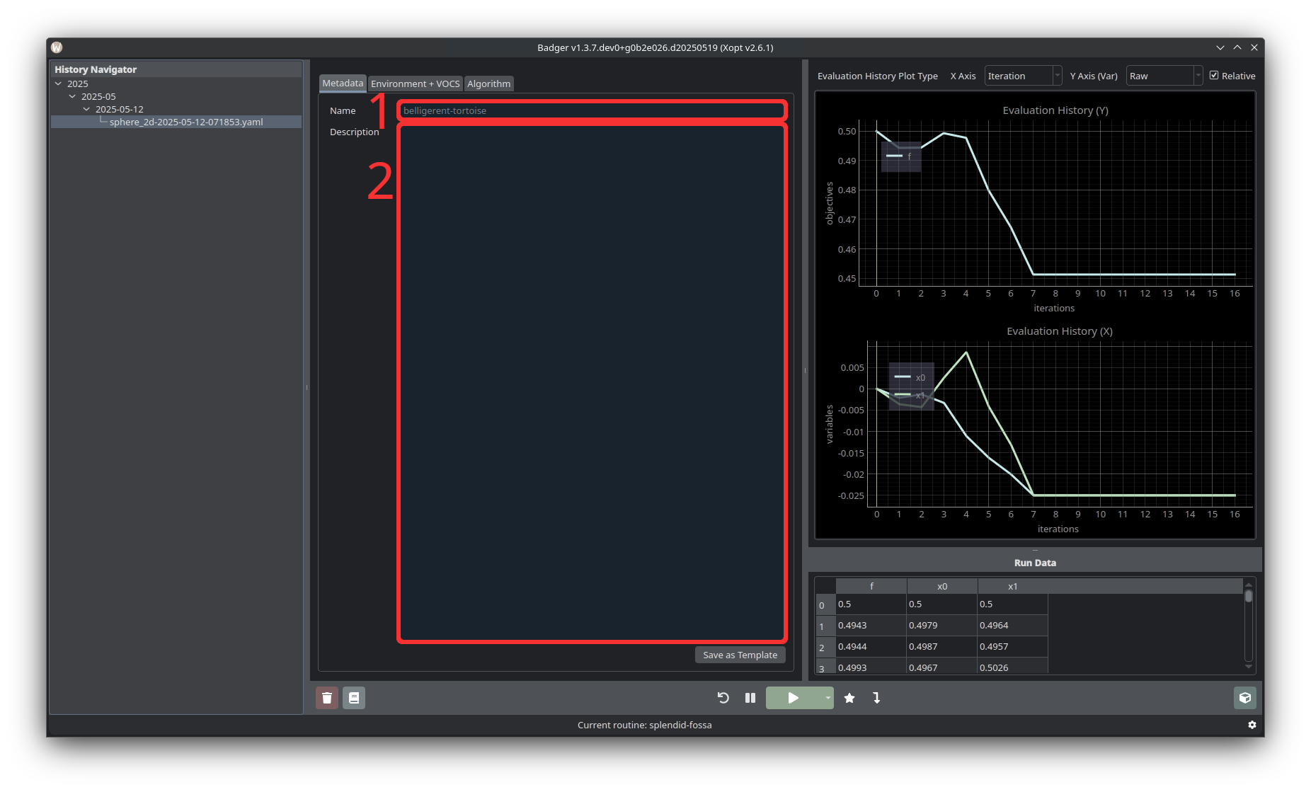
Metadata includes a name (1) and description (2) for the optimization routine. Beneath the description there is also a button to save the current run configuration as a template.
To Define a New Optimization Routine
-
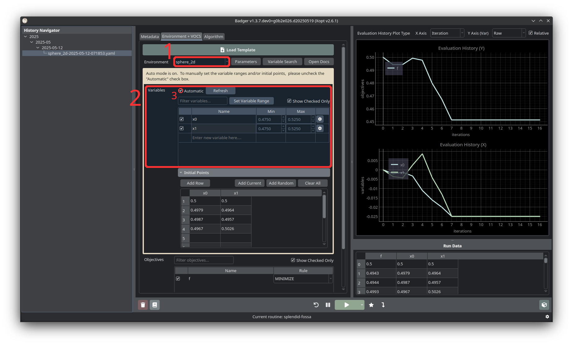
Start by selecting the target environment from the Environment dropdown. Click the Parameters button to expand the available environment parameters.
-
From the “Variables” table select devices to be optimized. The variables table shows all the variables which have been included in the selected environment. You can also toggle the Show Checked Only checkbox to only display selected variables. If a device you’d like to try to optimize is not listed, you can scroll to the bottom of the table and enter a new PV. The Min and Max columns in the table show the bounds of the search space for optimization. If the Automatic checkbox above the table is checked, these bounds will be ± some percentage from the current value. Clicking Set Variable Range will open a dialog window showing that ratio, and an option to select either relative to current or relative to the full variable range. Unchecking Automatic allows you to manually set variable ranges by editing the values in the Min and Max columns.
-
If the “Automatic” checkbox is checked, selecting a variable will automatically add a set of initial points. By default, these will be the current value followed by three random points within a fraction of the variable bounds centered around the current value. If Automatic is not checked, or to adjust the initial points, you can use the Add Current and Add Random buttons to configure your own initial points.
-
Select an objective from the “Objectives” table. Make sure to select whether the objective should be maximized or minimized! Currently only single objective optimization is available, but multi-objective optimization will be supported in the future.
-
Add constraints and observables. Beneath the Objectives table is a collapsable More section, which allows you to add Constraints and Observables. The constraints and observables available for selection are based on the selected environment.
-
Choose an optimization algorithm. There are several different optimization algorithms available within the Badger GUI. Generally, expected improvement and Nelder-Mead are good choices for online accelerator optimization. To select an algorithm navigate to the "Algorithm" tab.
-
Metadata: Provide a name and description for your optimization routine.
Running the Optimization
Once the environment, variables, objectives, and algorithm (and any optional constraints and observables) have been defined, the optimization can be started by pressing the green run button (5) at the lower center of the GUI. Badger will begin by measuring the objective at the initial points specified in the Initial Points table, and will then begin to optimize the selected variables using the chosen algorithm. When the scan is active, the green run button will turn into a red stop button.
- Once the scan has started, it can be paused/resumed using the play/pause button (4) to the left of the run button.
- To end the optimization run, press the red stop button (5).
After ending the optimization, you may want to take some sort of action on the variables/devices being optimized. Depending on the algorithm selected, the last point/state sampled may not be the best that was found during the optimization run. To select the best configuration of variables that was measured, press the star button titled Jump to Optimal (6) to the right of the stop/start button. Alternatively, clicking any point in the optimization plot will highlight the variable values at that point in the scan. Once you’ve chosen the solution you’d like to implement, press Dial in solution (7) to set devices to the selected values.
To reset all the variables to their values at the beginning of the scan, press the Reset Environment button (3).
Pressing the extensions button (8) will allow opening extension windows such as BOVisualizer and ParetoFrontViewer.
Pressing the delete button (1) will delete the stored run data from the History Navigator panel and on disk. Pressing the log button (2) will save the current run's log to the configured logbook directory.
While the optimization is running, the values of the variables, objectives, and (if selected) constraints and observables will be plotted in the plot section in the top right corner of the GUI. By default, the X-Axis displays the number of optimization iterations, and the Y-Axis for the variables plot is relative to each variable’s starting value. These options can be changed from the GUI via options in the top right corner, above the plots.
Advanced topics
Specify variable range
Each optimzation variable must have defined bounds that specify the valid search space. These ranges serve dual purposes: they constrain the optimization algorithm to explore only physically meaningful parameter values, and they enforce safety limits to prevent damage to the equipment. Variable ranges are defined in the Environment + VOCS section.
Incorporate algorithm parameters
Algorithm hyperparameters control how Xopt optimization algorithms explore the parameter space. These are distinct from the optimization variables (the machine parameters being tuned) and are algorithm-specific settings. These can be specified under Algorithm section. In Bayesian Optimization, hyperparameters include exploration parameter (beta) and maximum number of iterations (max_iter).
Check variable readout
Variable setters and getters may operate on different process variables (PVs). For example, magnet control typically sets via BCTRL but reads via BACT. Since Badger saves initial values using the getter and restores using the setter, reading BACT but writing to BCTRL during restoration may not return the system to its original state. Configure getters to read the same PV type as setters (preferably BCTRL for both) to ensure accurate save/restore functionality.
Delayed observation
Accelerator control systems require time to settle after parameter changes. Reading observables before the system reaches steady state would give the optimization algorithm misleading data. Badger environments can implement configurable wait times to specify delays between applying new variable values and reading measurements. These parameters allow users to adjust settling behavior without modifying code, ensuring measurements always reflect true steady-state performance. Implementation details will vary by facility.
In Badger, under Environments + VOCS, we have -
- trim_delay: This is time in seconds to wait after setting variables before starting data collection (LCLS-specific)
- validate_variable_set: If True, the program will wait to make sure variables reach their desired values (up to 'check_var_timeout') before starting the 'trim_delay'
- check_var_timeout: Timeout in seconds for checking if variables have reached target values