Tutorial

Heads-up

Make sure you have Badger installed and setup.

In this short tutorial, we are going to launch Badger in GUI mode, create a routine using the default sphere_2d environment shipped with Badger that optimize the following toy problem:

$$\begin{aligned} & \underset{x_0,\ x_1}{\text{maximize}} & & x_0^2 + x_1^2 \\ & \text{subject to} & & x_i \in [-1, 1], \; i = 0, 1. \end{aligned}$$

Then we'll customize the sphere_2d environment a bit to add one more variable and shape a sphere_3d environment, configure Badger so that it saves data to the directories we specify, create our second routine based on the new sphere_3d environment and finally run a new optimization on the problem below:

$$\begin{aligned} & \underset{x_0,\ x_1,\ x_2}{\text{minimize}} & & x_0^2 + x_1^2 + x_2^2 \\ & \text{subject to} & & x_0 \in [0, 1],\ x_1 \in [-1, -0.5],\ x_2 \in [0.5, 1] \; \end{aligned}$$

Let's get started.

Launch the Badger GUI

Run the following command in your terminal to launch the Badger GUI (assume you are in the python environment in which Badger was installed):

badger -g

Badger will ask if this is your first time using it. Either type a y and press Enter, or simply press Enter to fill out the default configuration values.

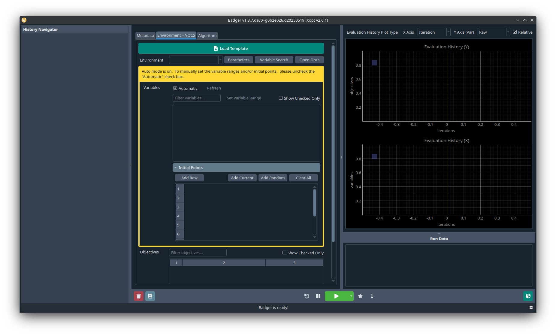
When it finishes writing the default config, you should be able to see the main GUI like below:

Run your first optimization

Before you can run the optimization, you need to set up the environment, VOCS, and algorithm. For your first routine, let's select the expected_improvement generator¹ in the Algorithm section. In the Environment + VOCS section, select the sphere_2d environment that's shipped with Badger.

Now we can shape our optimization problem by configuring the VOCS. Click the blank cell on top of the checkboxes in the variable table to include all the variables. If automatic mode is enabled, the Initial Points table should populate after this action. If it's not enabled, click the Add Current button in the Initial Points section to add the current values of the variables as the initial points where the optimization starts from. You of course can add more initial points as you wish but for now let's keep it simple -- we only start the run from the current values. Finally check the f observable shown in the objectives table and change the rule (direction of the optimization) to MAXIMIZE, this means we'll maximize f instead of minimize it (which is the default setting).

Now go ahead and click the green Run button, feel free to pause/resume the run anytime by clicking the button to the left of the run button, and click the run button (should be turned red now) again to terminate the run.

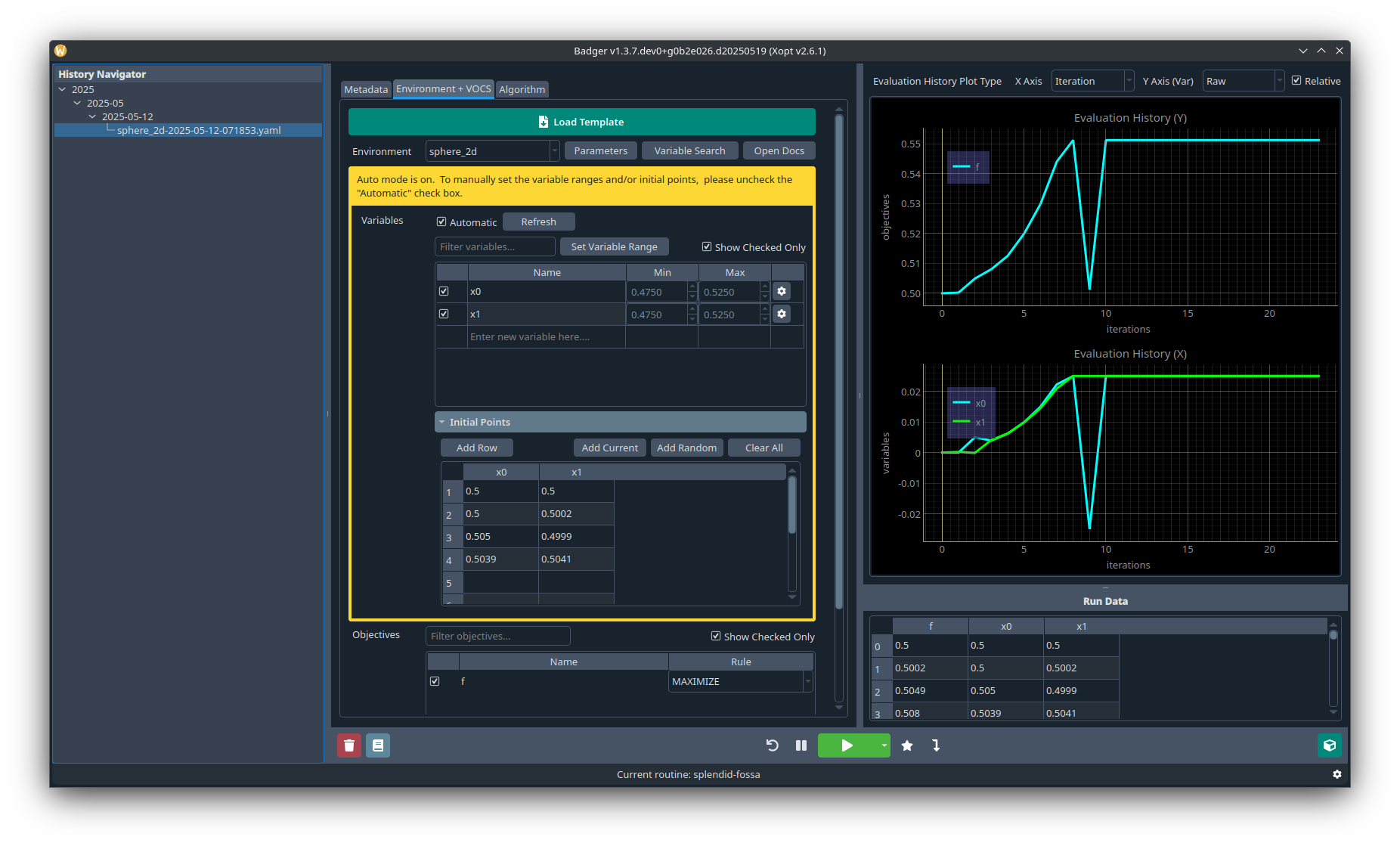
Congrats! You just run your very first routine in Badger!

Customize the environment

Now it's time to do some more serious stuff -- such as performing optimization on your own optimization problem. In order to do that, we need to create our own custom environment (and optionally, the corresponding interface).

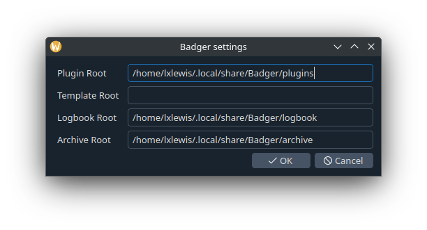
First let's point Badger to a new folder where we would like to store our custom plugins, if necessary. At the bottom right of the Badger GUI window is a settings cog. When clicked it will open a popup to configure the Badger plugin root, logbook root, and archive root. The default folders should be reasonable, but these can be changed to suit your needs, if the defaults are difficult to access. See the configuration page for more information.

In this example, we will be making an extension of the sphere_2d problem in 3 dimensions. Create a folder named sphere_3d in the environments folder beneath the plugin root. Then create the following files inside that sphere_3d folder:

• The main python script:

__init__.py

from badger import environment


class Environment(environment.Environment):

    name = 'sphere_3d'  # name of the environment
    variables = {  # variables and their hard-limited ranges
        'x0': [-1, 1],
        'x1': [-1, 1],
        'x2': [-1, 1],
    }
    observables = ['f']  # measurements

    # Internal variables to store the current values of
    # the variables and observables
    _variables = {
        'x0': 0.0,
        'x1': 0.0,
        'x2': 0.0,
    }
    _observations = {
        'f': None,
    }

    # Variable getter -- tells Badger how to get current values of the variables
    def get_variables(self, variable_names):
        variable_outputs = {v: self._variables[v] for v in variable_names}

        return variable_outputs

    # Variable setter -- how to set variables to the given values
    def set_variables(self, variable_inputs: dict[str, float]):
        for var, x in variable_inputs.items():
            self._variables[var] = x

        # Filling up the observations
        f = self._variables['x0'] ** 2 + self._variables['x1'] ** 2 + \
            self._variables['x2'] ** 2

        self._observations['f'] = [f]

    # Observable getter -- how to get current values of the observables
    def get_observables(self, observable_names):
        return {k: self._observations[k] for k in observable_names}

• The config file:

configs.yaml

---
name: sphere_3d
description: "3D sphere test environment"
version: "0.1"
dependencies:
  - torch
  - badger-opt

• And an optional readme:

README.md

# 3D Sphere Test Environment for Badger

## Prerequisites

## Usage

Now relaunch Badger GUI, you should be able the see the new custom environment we just created in the dropdown menu in the environment selector.

Run your second optimization

Now it's time to create our new routine with the newly created sphere_3d environment. This follows the same process as the earlier example. Select the sphere_3d environment and select the same algorithm as before. For this example, we'll change the variable ranges according to our target problem. We'll also change the initial point so that the optimization won't start with the best solution. Since our second problem is a minimization one, remember to change the direction of f to MINIMIZE.

Press Run and stop whenever you feel right, you should see some optimization curves like this:

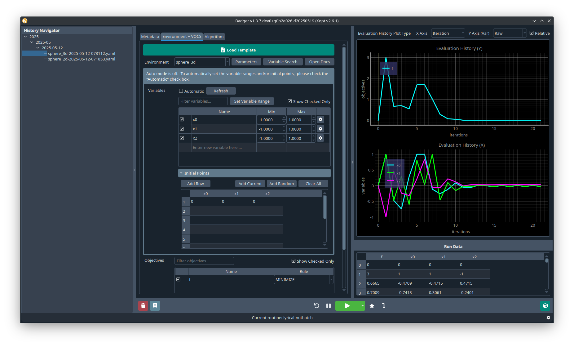
Congrats! You have accomplished the Badger GUI tutorial! Hope that by this point you already have some feelings about what Badger is and how Badger works. You can continue to the guides to adapt Badger to your own optimization problem! Please reach out to the official mailing list or Slack channel by following the links in the footer if you have any questions or need advice. If you encounter a bug please make an issue on the Badger GitHub repository. Good luck!

Footnotes

1. Term in Xopt, means algorithm ↩