Pareto front viewer
Overview
The Pareto front viewer extension allows for an interactive graphical interface for visualizing the Pareto front of a multi-objective optimization problem in both objective and variable spaces.
Usage
The extension can be used both statically and dynamically during or after a Badger optimization run. When used during a Badger optimization, the plots will update at a set interval in real time according to the variables and plot options set. Any plot options, reference points, and variables are saved throughout the use of that instance of the Pareto front viewer extension and are lost when the window is closed.
Constraints
The Pareto front viewer extension requires a Badger optimization run that uses an algorithm that utilizes the Xopt MOBOGenerator and that has 2 or more objectives defined in the optimization problem. The extension will not be available for single-objective optimizations and is only compatible with the mobo algorithm currently.
Tutorial
Step 1: Start Badger optimization
First step to use the Pareto front viewer is to use the Badger UI to run through an optimization using a compatible algorithm.
Once you have a converged on a solution or have stopped the optimization after a certain number of iterations, you can visualize the model by opening the Pareto front viewer extension.
Step 2: How to access the extension
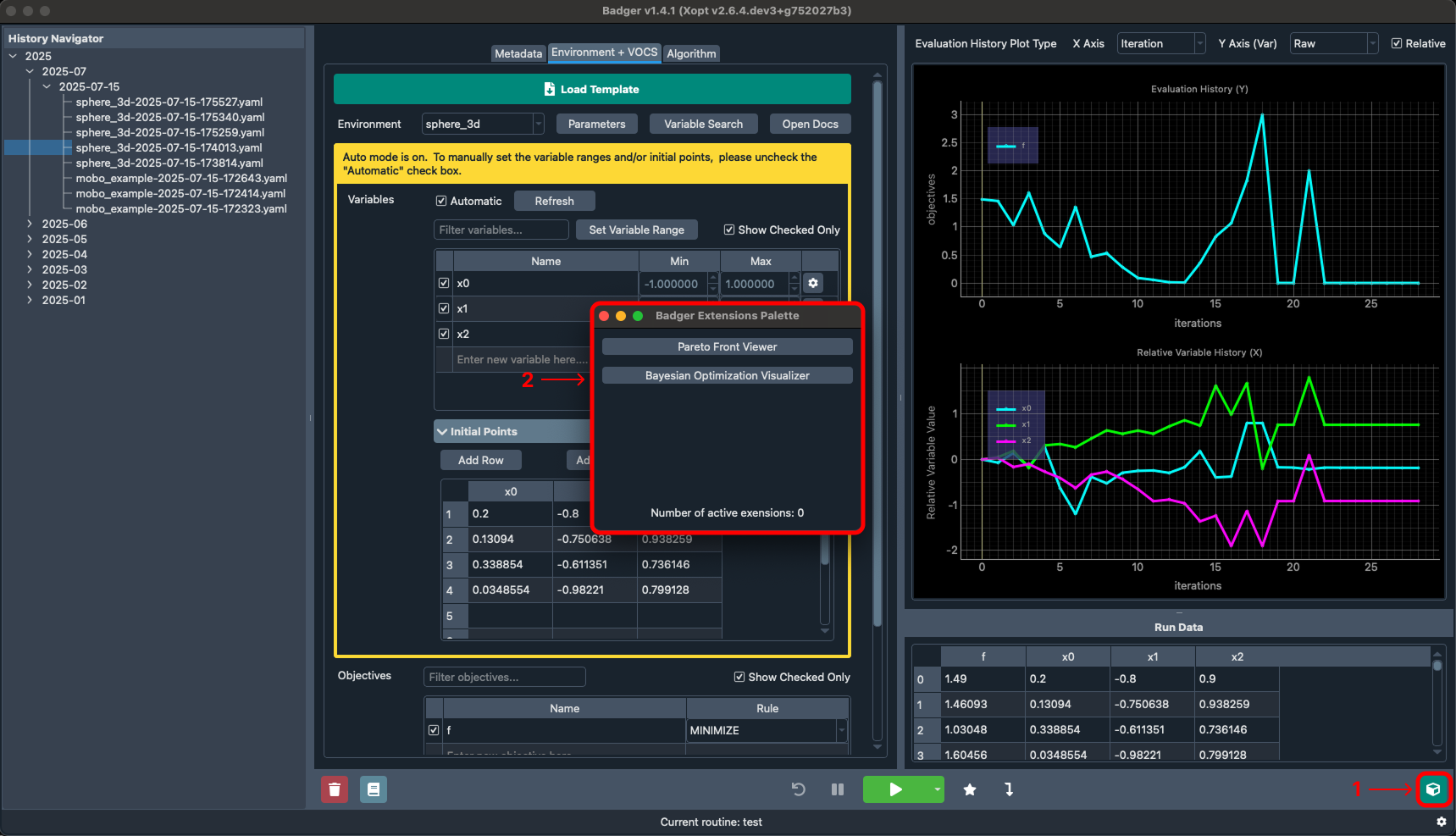
Description:
1 - Access the Badger extensions palette by clicking the icon in the bottom right
2 - The Badger extensions palette contains all extensions included by default with Badger Note: not all extensions are applicable to every optimization configuration
3 - Access the Pareto front viewer extension by clicking the corresponding option within the Badger extensions palette
Step 3: Pareto front viewer controls
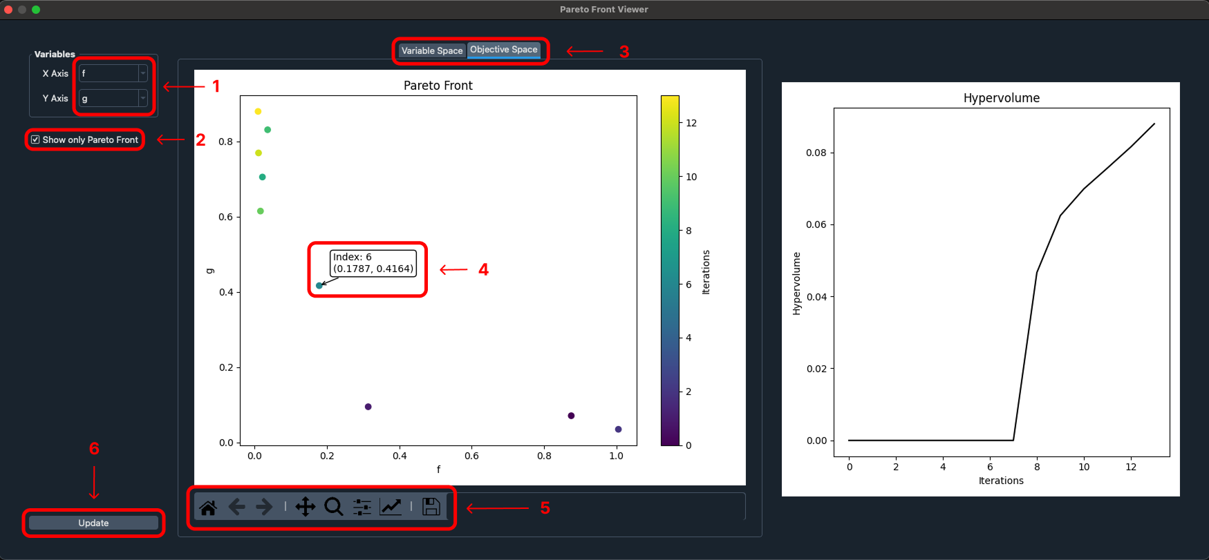
Description:
1 - Change the variables or objectives that are being plotted by the X and Y axes within the extension depending on the selected type of plot.
2 - To only show the data points that are included in the Pareto front, you can enable the "Show only Pareto Front" option and the charts will update to show those data points.
3 - There are two separate charts that visualize the Pareto front data in different ways: one in an objective space and one in the variable space. When selecting either of these charts through the tabs at the top of the extension, the corresponding data will be displayed. The X and Y axes plotted within the chart will update automatically according to the selected chart type.
4 - The charts within the extension are interactive through mouse inputs and can display additional information.
The possible actions are as follows:
Left Click- Select a data point to view both the coordinate values in the selected space and the index of the iteration that the data point corresponds to within the optimization run.Right ClickorMiddle Click- Will reset the view to the default state.Scroll- Zoom in and out of the chart.
5 - For additional interaction options, you can also use the Matplotlib navigation toolbar to modify the current view or export the current plot.
6 - The Pareto front viewer extension will automatically update the charts reactively upon any changes however, if at any point you believe the plots are out of sync then you can forcefully update the plots using the update button
Charts explanation
The leftmost chart is able to visualize the optimization run data in either the objective space or the variable space, depending on the selected tab. When the objective space tab is selected, the chart will display the values of the objectives selected for each axes as the optimization progressed. When the variable space tab is selected, the chart will display the same information for the input variables. For both of the charts, each of the data points are color-coded based on the index of the corresponding iteration within the optimization run. When the "Show only Pareto Front" option is enabled, the chart will only display the data points that are directly a part of the Pareto front in the selected space.
The rightmost chart is a plot of the hypervolume as it evolves over the course of the optimization run. The hypervolume is a measure of the volume of the space covered by the Pareto front.